Chapter 11 Round up
This chapter consists of some thoughts I considered relevant for this course but which did not seem to fit well in any of the other chapters.
11.1 Comparing models
The package plotmo provides nice functionality to plot diffent classes of models. We use it to compare a few models introduced in the previous chapters: 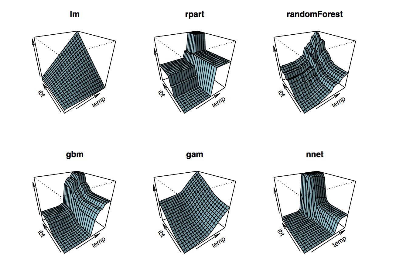
I think this graph is a nice summary of what we leared in this course. We can characterize the models by:
- How smooth the fitted surface is. Linear models are smooth by nature (if there are no dummy variables involved), random forest (rpart) are just piecewise constant. Random forest are smoother than trees because they are aggregated trees. Ignore gbm for now and note that neural nets are also rather smooth.
- How flexible they are: Linear models are not very flexible, gams are only additive, so no interaction effects, trees can have interaction effects, so do random forests.
This is a rough classification, but it grasps the general pattern.
11.2 Exercises Take-aways
Creating Formulas Task (Series 11): Generate a R-formula for a cubic penalized regression model that accounts for all 3-way interactions.
From ?formula
The ^ operator indicates crossing to the specified degree. For example (a+b+c)^2 is identical to (a+b+c)*(a+b+c) which in turn expands to a formula containing the main effects for a, b and c together with their second-order interactions.
library(sfsmisc)
formula <- wrapFormula(
  logO3 ~.,
  data = data,
  wrapString = "poly(*, degree = 3" # polynomial
)
update(formula, logO3 ~ .^3) # three way interaction
Matrix Multiplication
- You can’t multiply data frames. No way. Use
as.matrixto convert. - Don’t forget the intercept in the model frame.
Other
R is vectorized. Before writing complicated
map()stuff, think about whether it is possible to do all calculations vectorised. Compare exercise series 8.Scaling and Transformations: If the response or in fact any variable is highly skewed, use the log as a first aid transformation to for efficiency. Also, some methods such as neural networks work better with scaled predictors. Another category are methods such as lasso or ridge regression, where it is beneficial for interpretability to scale the variables.
Accessing model parameters
When calculating the degrees of freedom, e.g. for the mallows cp, never use someghing like `length(coef(fit))`` as \(p\), since this will only work for linear models. For additive models for example, this will give you the number of soothing terms used, which is not equivalent to the degrees of freedom. Instead, use
fit$df.residualWhich is available for many classes of fitted models, i.e. also GAMs. Also, often it is not necessary to compute something like the residual standard error, since you can conveniently access it via
summary(fit)$sigmaAlso, do sanity checks for your results. A qick plot(unlist(cps)) for example can show you the various values cp takes for different model vs. their index. As with cross validation, you know that the curve must be somehow convex.
Inconsistent S3 generics
Unfortunately, not all S3 generics do feature the same argument names. This is particularly dangerous when using ... to pass arguments. For example, different predict methods do not use the same argumet for new data. Some use newdata, others data etc.
Programming: Fail Fast and debug
Unit testing on the ways costs next to nothing. Don’t wait testing your functions until you are done with the whole exam. Examples are
- boostrapping: Test whether regression coefficients are exactly the true coefficients when no noise has been added. Otherwise, check whether they are reasonable.
- Test dimensions of matrices you use.
- Test whether values you obatain are plausible
- use
browser()extensively, even when writing a function, not just to debug it.
Do not assign fitted values to initial data frame This is dangerous since you are probably doing something like
fit <- lm(y~., data = data)
data$yhat <- predict(fit, data)
# you may do next
glm(y~., data = data, family = binomial) # yhat will be predictor now
** Series 3 - Non-parametric Regression** - The smoother matrix \(S\) does not change if the x values are fix. - The bias is \(E[f(x) - \hat{f}(x)]\), so use the true values without the added noise for \(f(x)\). - diag(), t() and %*%. - Be careful with formulas and write them first donw on paper. E.g. \(\hat{sd(\hat{m}(x))}\). - Don’t confuse variance and standard error. - Simultanous coverage calculations of many simulations can be done simpler than true > lower_ci & true > upper_ci, namely via abs(m(x) - m_hat(x)) <= 1.96 * sd(m_hat), which can be vectorised with matrices. To be verbose, use replicate(nrep, m(x)) to create a matrix with nrep columns, which all just contain m(x).
#' Estimate the coverage
#'
#' Estimates how many times a confidence interval over all x contains the
#' true value.
#' @param est A matrix with nrep predictions for each observed x
#' @param se A matrix with the corresponding to `est` with standard deviations
#'   at each x.
#' @param true A vector with the n true values (no noise added).
est_coverage <- function(est, se, true = m(x)) {
  inside <- sum(
    apply(abs(est - replicate(ncol(est), true)) <= 1.96 * se, 2, all)
  )
  inside
}
Series 5
Only because there is no exported S3 generic (e.g. for predict()), it does not mean there is none!
11.3 Cheatsheet
- The boostrapped confidence intrevals are
\[[2 \hat{\theta} - q_{1-\alpha/2}, 2\hat{\theta}- q_{\alpha/2}]\] * You can represent a matrix multiplication as a sum of outer product multiplications whereas \(x_i\) is one column from the maxtix \(X_{n \times p}\) and has dimensions \(n \times 1\) \[ (X'X) = \sum\limits_{i = 1}^p x_i x_i'\]
- Scalars can be moved out of a more complicated matrix multiplication. \(ab'A^{-1}ab'A^{-1} = (b'A^{-1}a)ab'A^{-1}\)
- \((X(X'X)^{-1}X')_{ii} = x_i'(X'X)^{-1}x_i\)
- \(uDu'\) can be rewritten as \(\sum\limits_{j = 1}^p d_j u_j u_j'\) if you think of the matrices a row vectors and each element of such a vector is a vector itself (Credits @NG).
Always sort the data when working with smoother matrices.
The short cut for leave one out CV with linear fitting operators is
\[ n^{-1} \sum\limits_{i = 1}^n \Big(\frac{y_i - \hat{m}(x_i)}{1-S_{ii}}\Big)^2\]
- use roxygen comemnts instead of normal comments since the propagate to new line
- You can do k-fold CV with
i in 0:kfold-1, where M is the size of the fold.
test_ind <- (i * M + 1):((i + 1) * M)