Chapter 6 Bootstrap
- Bootstrap can be summarized as “simulating from an estimated model”
- It is used for inference (confidence intervals / hypothesis testing)
- It can also be used for estimating the predictive power of a model (similarly to cross validation) via out-of-bootstrap generalization error
6.1 Motivation
Consider i.i.d. data. \[ Z_1, .. Z_n \sim\ P \;\; with \; \;Z_i = (X_i, Y_i)\] And assume a statistical procedure \[ \hat{\theta} = g(Z_1, ..., Z_n) \] \(g(\cdot)\) can be a point estimator for a regression coefficient, a non-parametric curve estimator or a generalization error estimator based on one new observation, e.g. \[ \hat{\theta}_{n+1} = g(Z_1, ..., Z_{n}, Z_{new}) = (Y_{new} - m_{Z_1, ..., Z_{n}}(X_{new}))^2 \] To make inference, we want to know the distribution of \(\hat{\theta}\). For some cases, we can derive the distribution analytically if we know the distribution \(P\). The central limit theorem states that the sum of random variables approximates a normal distribution with \(n \rightarrow \infty\). Therefore, we know that the an estimator for the mean of the random variables follows the normal distribution. \[ \hat{\theta}_{n} = n^{-1}\sum x_i \sim N(\mu_x, \sigma_x^2 / n) \; \; \; n \rightarrow \infty \] for any \(P\). However, if \(\hat{\theta}\) does not involve the sum of random variables, and the CLT does not apply, it’s not as straightforward to obtain the distribution of \(\hat{\theta}\). Also, if \(P\) is not the normal distribution, but some other distribution, we can’t find the distribution of \(\hat{\theta}\) easily. The script mentions the median estimator as an example for which the variance already depends on the density of \(P\). Hence, deriving properties of estimators analytically, even the asymptotic ones only, is a pain. Therefore, if we knew \(P\), we could simply simulate many times and get the distribution of \(\hat{\theta}\) this way. That is, draw many \(({X_i}^*, {Y_i}^*)\) from that distribution and compute \(\hat{\theta}\) for each draw.
The problem is that we don’t know \(P\). But we have a data sample that was generated from \(P\). Hence, we can instead take the empirical distribution \(\hat{P}\) that places probability mass of \(1/n\) on each observation, draw a sample from this distribution (which is simply drawing uniformly at random from our sample with replacement) and compute our estimate of interest from this sample. \[ \hat{\theta}^{*} = g({Z_1}^{*}, ..., {Z_{new}}^{*})\] We can do that many times to get an approximate distribution for \(\hat{\theta}\). A crucial assumption is that \(\hat{P}\) reassembles \(P\). If our data is not i.i.d, this may not be the case and hence bootstrapping might be misleading. Below, we can see that i.i.d. sampling (red line) reassembles the true distribution (black line) quite well, whereas biased sampling (blue line) obviously does not. We produce a sample that places higher probability mass on the large (absolute) values.
library("tidyverse")
pop <- data_frame(pop = rnorm(10000) * 1:10000)
iid <- sample(pop$pop, 1000, replace = TRUE) # sample iid

# sample non-iid: sample is biased towards high absolute values
ind <- rbinom(10000, size = 1, prob = seq(0, 1, length.out = 10000))
not_iid <- pop$pop[as.logical(ind)] # get sample
not_iid <- sample(not_iid, 1000, replace = TRUE) # reduce sample size to 1000

out <- data_frame(iid = iid, not_iid = not_iid) %>%
  gather(type, value, iid, not_iid)
ggplot(out, aes(x = value, color = type)) +
  geom_density() +
  geom_density(aes(x = pop, color = NULL), data = pop)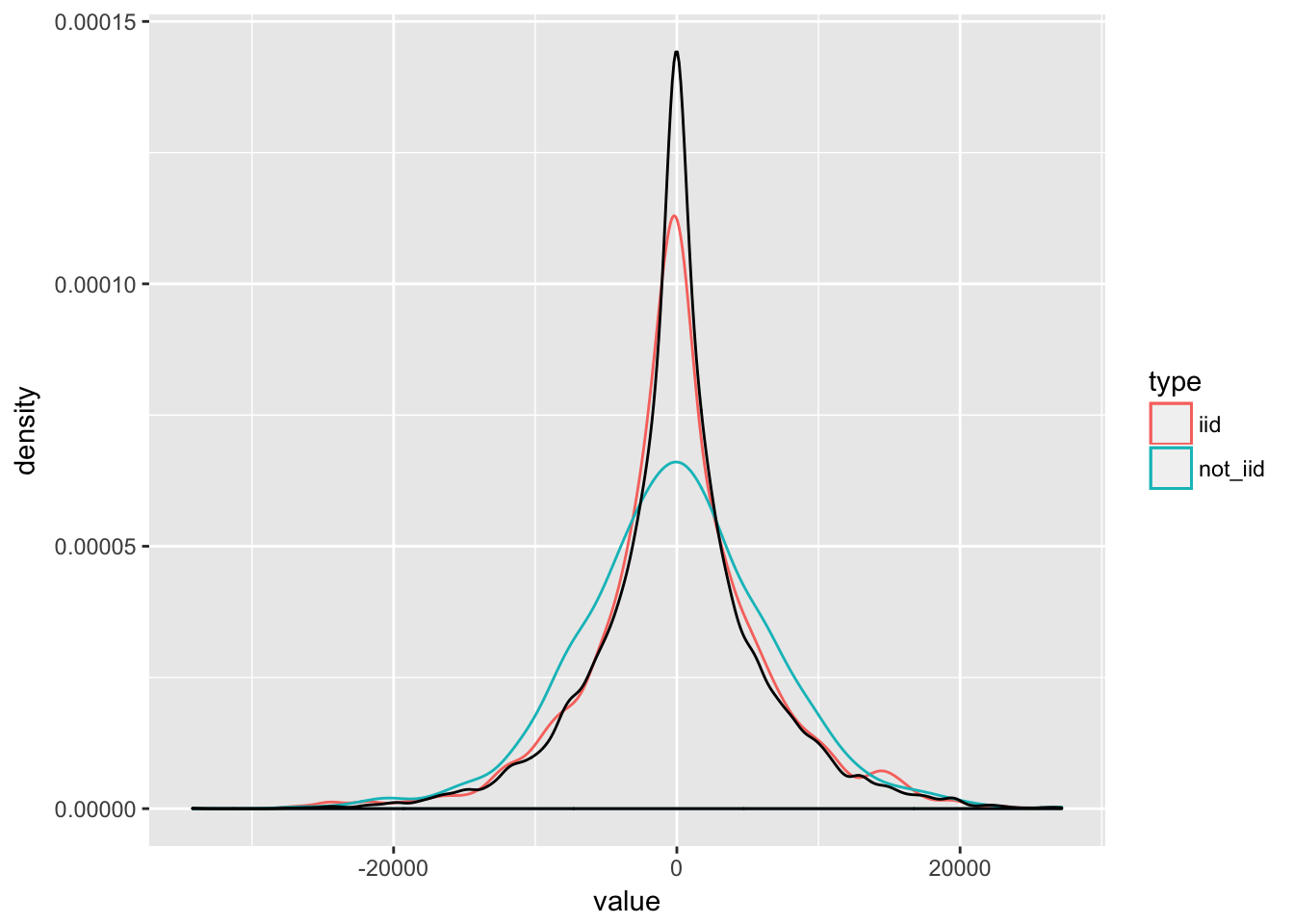
We can summarize the bootstrap procedure as follows.
- draw a bootstrap sample \({Z_1}^{*}, ..., {Z_{n}}^{*}\)
- compute your estimator \({\hat{\theta}}^*\) based on that sample.
- repeat the first two steps \(B\) times to get bootstrap estimators \({\hat{\theta}_1}^*, ..., {\hat{\theta}_B}^*\) and therefore an estimate of the distribution of \(\hat{\theta}\).
Use the \(B\) estimated bootstrap estimators as approximations for the bootstrap expectation, quantiles and so on. \(\mathbb{E}[\hat{\theta}^*_n] \approx B^{-1}\sum\limits_{j = 1}^n \hat{\theta}^{* j}_n\)
6.2 The Bootstrap Distribution
With \(P^*\), we denote the bootstrap distribution, which is the conditional probability distribution introduced by sampling i.i.d. from the empirical distribution \(\hat{P}\). Hence, \(P^*\) of \({\hat{\theta}}^*\) is the distribution that arises from sampling i.i.d. from \(\hat{P}\) and applying the transformation \(g(\cdot)\) to the data. Conditioning on the data allows us to treat \(\hat{P}\) as fixed.
6.3 Bootstrap Consistency
The bootstrap is is called consistent if \[ \mathbb{P}[a_n(\hat{\theta} - \theta) \leq x ] - \mathbb{P}[a_n(\hat{\theta}^* - \hat{\theta}) \leq x ] \rightarrow 0 \;\; (n \rightarrow \infty)\] Consistency of the bootstrap typically holds if the limiting distribution is normal and the samples \(Z_1, .., Z_n\) are i.i.d. Consistency of the bootstrap implies consistent variance and bias estimation:
\[ \frac{Var^* (\hat{\theta}^*)}{Var(\hat{\theta})} \rightarrow 1\] \[ \frac{\mathbb{E}^* (\hat{\theta}^*) - \hat{\theta}}{\mathbb{E}(\hat{\theta}) - \theta} \rightarrow 1\] You can think of \(\theta\) as the real parameter and \(\hat{\theta}\) as the estimate based on a sample. Similarly, in the bootstrap world, \(\hat{\theta}\) is the real parameter, and \(\hat{\theta}^*_i\) as an estimator of the real parameter \(\hat{\theta}\). The bootstrap world is an analogue of the real world. So in our bootstrap simulation, we know the true parameter \(\hat{\theta}\). From our simulation, we get many \(\hat{\theta}^*_i\) and can find the bootstrap expectation \(\mathbb{E}[\hat{\theta}^*_n] \approx B^{-1}\sum\limits_{j = 1}^n \hat{\theta}^{* j}_n\). The idea is now to generalize from the boostrap world to the real world, i.e. by saying that the relationship between \(\hat{\theta}^*\) and \(\hat{\theta}\) is similar to the one between \(\hat{\theta}\) and \(\theta\).
A simple trick to remember all of this is:
- if there is no hat, add one
- if there is a hat, add a star.
6.4 Boostrap Confidence Intervals
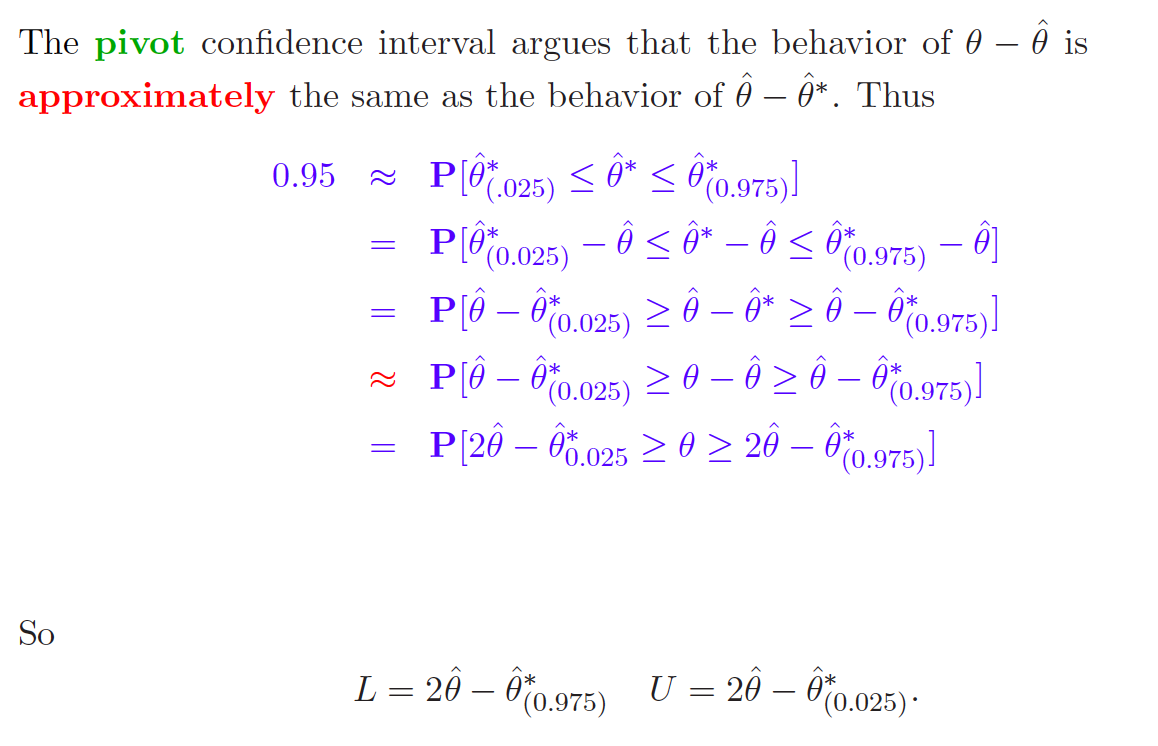
Note that there confidence intervals are not simply taking the quantiles of the bootstrap distribution. The trick is really to make use of the analogy between the real world and the boostrap world. So when we see our bootstrap expectation \(\mathbb{E}[\hat{\theta}^*_n]\) is way higher than \(\hat{\theta}\), then we also should believe that our \(\hat{\theta}\) is higher than \(\theta\). The above procedure accounts for that.
6.5 Boostrap Estimator of the Generalization Error
We can also use the bootstrap to estimate the generalization error. \[ \mathbb{E}[\rho(Y_{new}, m^*(X_{new}))] \]
- We draw a sample \(({Z_1}^*, ..., {Z_n}^*, Z_{new})\) from \(\hat{P}\)
- We compute the bootstrapped estimator \({m(\cdot)}^*\) based on the sample
- We estimate \(\mathbb{E}[\rho(Y_{new}, {m^*(X_{new})}^*)]\), which is with respect to both training and test data.
We can rewrite the generalization error as follows: \[ \mathbb{E}[\rho(Y_{new}, m^*({X_{new}}^*))] = \mathbb{E}_{train}[E_{test}[\rho({Y_{new}}^*, m^*({X_{new}}^*))| train]]\] Conditioning on the training data in the inner expectation, \(m(\cdot)\) is non-random / fixed. The only random component is \({Y_{new}}^*\). Since we draw from the empirical distribution and place a probability mass of \(1/n\) on every data point. we can calculate the inner (discrete) expectation easily via \(\mathbb{E}(X) = \sum\limits_{j = 1}^n p_j * x_j = n^{-1} \sum\limits_{j = 1}^n x_j\). The expectation becomes \[ \mathbb{E}_{train}[n^{-1}\sum\rho(Y_{i}, m^*(X_{i}))] = n^{-1}\sum\mathbb{E}[\rho(Y_{i}, m^*(X_{i}))]\]
We can see that there is no need to draw \(Z_{new}\) from the data. The final algorithm looks as follows:
- Draw \(({Z_1}^*, ..., {Z_n}^*)\)
- compute bootstrap estimator \({\hat{\theta}}^*\)
- Evaluate this estimator on all data points and average over them, i.e \(err^* = n^{-1} \sum \rho(Y_i, m^*(X_i))\)
- Repeat steps above B times and average all error estimates to get the bootstrap GE estimate, i.e. \(GE^* = B^{-1} \sum {err_i}^*\)
6.6 Out-of-Boostrap sample for estimating the GE
One can criticize the GE estimate above because some samples are used in the test as well as in the training set. This leads to over-optimistic estimations and can be avoided by using the out-of-bootstrap approach. With this technique, we first generate a bootstrap sample to compute our estimator and then use the remaining observations not used in the bootstrap sample to evaluate the estimator. We do that \(B\) times and the size of the test set may vary. You can see this as some kind of cross-validation with about 30% of the data used as the test set. The difference is that some observations were used multiple times in the training data, yielding a training set always of size n (instead of - for example \(n*0.9\) for 10-fold-CV).
6.7 Double Boostrap Confidence Intervals
Confidence intervals are almost never exact, meaning that \[\mathbb{P}[\theta \in I^{**}(1-\alpha)] = 1-\alpha + \Delta\] Where \(I^{**}(1-\alpha)\) is a \(\alpha\)-confidence interval. However, by changing the nominal coverage of the confidence interval, it is possible to make the actual coverage equal to an arbitrary value, i.e
\[ \mathbb{P}[\theta \in I^{**}(1-\alpha')] = 1-\alpha\] The problem is that \(\alpha'\) is unknown. But another level of bootstrap can be used to estimate \(\alpha\), denoted by \(\hat{\alpha}\), which typically achieves \[\mathbb{P}[\theta \in I^{**}(1-\hat{\alpha}')] = 1- \alpha + \Delta'\] with \(\Delta' < \Delta\)
To implement a double bootstrap confidence interval, proceed as follows:
- Draw a bootstrap sample \(({Z_1}^*, ..., {Z_n}^*)\).
- From this sample, draw B second-level bootstrap samples and compute the estimator of interest and one confidence interval \(I^{**}(1-\alpha)\) based on B second-level bootstrap samples.
- evaluate whether \(\hat{\theta}\) lays within the bootstrap confidence interval from a. \(cover^*(1-\alpha) = 1_{[\hat{\theta} \in I^{**}(1-\alpha)]}\)
- Repeat the above M times to get \(cover^{* 1}, ..., cover^{* M}\) and hence approximate \(\mathbb{P}[\theta \in I^{**}(1-\alpha)]\) with \[ p^*(\alpha) = M^{-1} \sum\limits_{m = 1}^M cover^{* m}\]
- Vary \(\alpha\) in all of the steps above to find \(\alpha'\) so that \(p^*(\alpha') = 1- \alpha\)
Question here (see Google docs)
6.8 Three Versions of Boostrap
- So far, we discussed the fully non-parametric bootstrap, which is simulating from the empirical distribution.
- On the other extreme of the scale, there is the parametric bootstrap.
- The middle way is the model-based bootstrap
6.8.1 Non-parametric Regression
We draw a bootstrap sample \(({Z_1}^*, ..., {Z_n}^*) \sim \hat{P}\), i.e. we sample from the empirical distribution data with replacement.
6.8.2 Parametric Boostrap
Here, we assume the data are realizations from a known distribution \(P\), which is is determined up to some unknown parameter (vector) \(\theta\). That means we sample \((Z_1, ..., Z_n) \sim P_{\hat{\theta}}\). For example, take the following regression model \(y = X\beta + \epsilon\) where we know the errors are Gaussian.
- We can estimate our regression model, obtain residuals and compute the mean (which is zero) and the standard deviation of them.
- To generate a bootstrap sample, we simulate residuals \(\epsilon^*\) from \(N(0, \hat{\mu})\) and
- Add them to our observed data, i.e. we obtain \(({Y_1}^*, ..., {Y_n}^*)\) from \(X\beta + \epsilon^*\). Hence, the final bootstrap sample we use is \((x_1, {Y_1}^*), ..., (x_1, {Y_n}^*))\) where the \(x_i\) are just the observed data.
- We can compute bootstrap estimates \(\hat{\beta}^*\), the bootstrap expectation \(\mathbb{E}^*[\beta*]\) as well as confidence intervals for the regression coefficients or generalization errors just as shown in detail above. The difference is only how the bootstrap sample is obtained.
Similarly, for time series data, we may assume an AR(p) model.
- Initializing \({X_0}^*, ..., {X_{-p+1}}^*\) with \(0\).
- Generate random noise \({\epsilon_1}^*, ..., {\epsilon_{n+m}}^*\) according to \(P_{\hat{\theta}}\).
- Construct our time series \({X_t}^* = \sum\limits_{j = 1}^p \hat{\theta}{X_{t-j}}^* + {\epsilon_t}^*\) \((X_1, ..., X_{n+m})\)
- Throw away the first \(M\) observations that were used as fade-in.
- Proceed with the B bootstrap samples \(({X_1}^*, ..., {X_n}^*)\) as outlined above for the non-parametric bootstrap to obtain coefficient estimates for \(\theta\), confidence intervals or estimating the generalization error of the model.
6.8.3 Model-Based Bootstrap
The middle way is the model based bootstrap. As with the parametric bootstrap, we assume to know the model, e.g. \(y = m(x) + \epsilon\) (where \(m(\cdot)\) might be a non-parametric curve estimator), but we do not make an assumption about the error distribution. Instead of generating \(\epsilon^*\) from the known distribution with unknown parameters (\(\epsilon^* \sim P_{\hat{\theta}}\), as in the parametric bootstrap)), we draw them with replacement from the empirical distribution. To sum it up, these are the steps necessary:
- Estimate \(\hat{m(\cdot)}\) from all data.
- Simulate \({\epsilon_1}^*, ..., {\epsilon_n}^*\) by drawing from \(\hat{P}\) with replacement.
- Obtain \(({Y_1}^*, ..., {Y_n}^*)\) from \(\hat{m}(x) + \epsilon^*\). As for the parametric bootstrap, the final bootstrap sample we use is \((x_1, {Y_1}^*), ..., (x_n, {Y_n}^*))\) where the \(x_i\) are just the observed data.
- Again, you can use the bootstrap samples as for the other two methods.
6.9 Conclusion
Which version of the bootstrap should I use? The answer is classical. If the parametric model fits the data very well, there is no need to estimate the distribution explicitly. Also, if there is very little data, it might be very difficult to estimate \(P\). On the other hand, the non-parametric bootstrap is less sensitive to model-misspecification and can deal with arbitrary distributions (? is that true?).