Chapter 10 Bagging and Boosting

Bagging stands for bootstrapping aggregating and

10.1 Bagging

Bagging works as follows: Consider a base procedure \[ \hat{g}(\cdot): \mathbb{R}^p \rightarrow \mathbb{R}\]

1. Draw a bootstrap sample \((Y_1^*, X_1^*), ..., (Y_1^*, X_n^*)\) and compute the bootstrap estimator \(\hat{g}(\cdot)^*\).
2. Repeat the above step \(B\) times yielding \(\hat{g}(\cdot)^{*1}, ..., \hat{g}(\cdot)^{*B}\) bootstrap estimators
3. Average the estimates to construct the bagged estimator: \[ \hat{g}_{Bag}(x) = n^{-1} \sum\limits_{i = 1}^B\hat{g}(\cdot)^{*i}\] Then, \(\hat{g}(\cdot)\) is nothing else than an approximation of the bootstrap expectation. \[\hat{g}(\cdot) \approx \mathbb{E}^*[g(x)^{*}]\] Note that the novel point is that we now use this approximation as an estimate of \(g(\cdot)\). However, \[\begin{equation} \begin{split} \hat{g}(\cdot)_{Bag} & = \hat{g}(\cdot) + \mathbb{E}^*[g(x)^{*}] - \hat{g}(\cdot) \\ & = \hat{g}(\cdot) + \text{bootstrap bias estimate} \end{split} \end{equation}\]

Instead of subtracting the bootstrap bias estimate, we are adding it! However, for trees for example, bagging reduces the variance of the estimate so much that the bias increase will not be strong enough to push the mean square error up. Let us consider a one-dimensional example.

The variance of an indicator function (which is a Bernoulli experiment) is given by \[ Var(1_{X>d}) = \mathbb{P}(X > d)(1 - (\mathbb{P}(X > d))\] If we assume \(X \sim N(0, 1)\) and \(d = 0\), \(\mathbb{P}(X > d) = 1 - \mathbb{P}(X<d) = 0.5\), so the above quantity is \(1/4\). For bagged trees, it turns out that the estimator is a product of probit functions \(\phi(d-X)\). Since it holds that \[ \text{if}\;\; X \sim F, \;\;F(X) \sim U\] the variance of random forest is \[Var(\phi(d-X)) = Var(U) = 1/12\] So the variance was reduced by a factor of 3.

10.2 Subagging

Subagging stands for sub-sampling and aggregation. It is different from bagging in that instead of drawing bootstrap samples of size \(n\), we only draw samples of size \(m < n\), that is \((X_1^*, Y_1^*), ..., (X_m^*, Y_m^*)\) but without replacement. It can be shown that for some situations, subagging with \(m = n/2\) is equivalent to bagging, hence, subagging is a cheap version of bagging.

Bagging (and subagging) have one drawback which is the lack of interpretability. In the script, there is a comparison between MARS and trees. Both subagging and bagging helps for trees, but does not help for MARS. How come? Remember that fitted values of trees are piece-wise constant. Bagging makes them smoother (and hence more like MARS). MARS yield a piece-wise linear function by nature. Trees have a high variance and hence the bias-variance trade-off can be optimized with bagging. MARS don’t have such a high variance, hence, optimization is not possible to the same extend.

10.3 \(L_2\)-Boosting

We saw bagging was a variance reduction technique. Boosting is a bias reduction technique. As with bagging there is a base estimator \(\hat{g}(\cdot)\). Then, you basically refit it to the residuals to reduce them many times. The concrete implementation is:

• Fit an estimator to the data and compute the residuals \[U_i = Y_i - \nu\hat{g}_1(x_i)\] where $< 1 $ is a tuning parameter. The smaller \(\nu\), the more explainable residuals you leave for suceeding estimators. Denote \(\hat{f}_1(x) = \nu g_1(x)\)

• For m = 2, 3, …, M: Fit the residuals to the data, i.e \[ (X_i, U_i) \rightarrow \hat{g}(x)\] Set \[ \hat{f}_m(x) = \hat{f}_{m-1}(x) + \nu \hat{g}_m(x)\] Compute the current residuals: \[U_i = Y_i - \hat{f}_m(x)\]

A small \(\nu\) can be interpreted as follows: You go into the right direction, but you do that slowly and you allow yourself to be corrected later.

Boosting can be useful in the context of thinning-out with trees, where you don’t have enough observations in the terminal nodes to continue. Boosting then comes up with a more complex solution by taking linear combinations of trees. For classificcation trees, you can also extend the tree by taking

Boosting can also be used for varible selection. For example, let \(\hat{g}\) be a GAM with one predictor. Then, for each variable fit such a gam and set \(f_1(x) = arg\min\limits_{\hat{g}_j(x) \; j =\{1, ..., p\}}\|Y - \hat{g}_j(x)\|\), i.e. take the the additive model that had the smallest residual sum of squares. Then, use the adjusted residuals from it and fit another \(p\) GAMs and select again the gam with the smallest RSS.

10.4 Some unfinished stuff

Let’s consider a simple one-dimensional example. If you have a cut-off at \(d\) (so for example for classification, \(X > d\) is classified as \(1\), \(X < d\) as \(0\)) and you take the mean over many bootstrap samples (which you do with random forests, where each tree has a potentially different \(d\)), with \(n \rightarrow \infty\) you get a smooth function (probably some form of a transformed binomial that is asymptotically normal)

one_mean <- function(d = 0, ...) {
  x <- rnorm(...)
  x_boolean <- x > d
  mean(x_boolean)
}

mean_sim <- rerun(1000, one_mean(n = 200)) %>%
  flatten_dbl()

ggplot(data_frame(mean = mean_sim), aes(x = mean)) +
  stat_ecdf(geom = "step")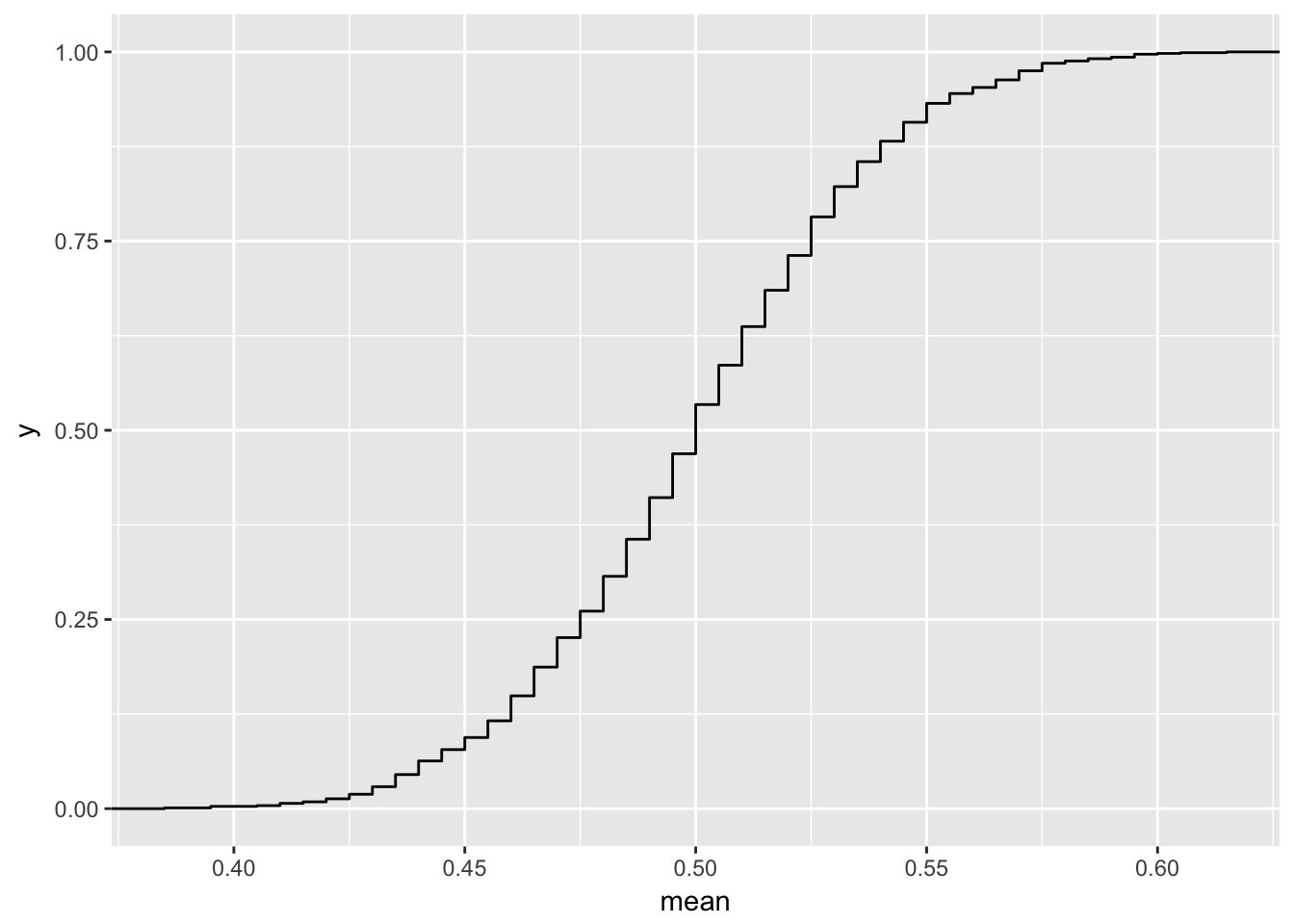

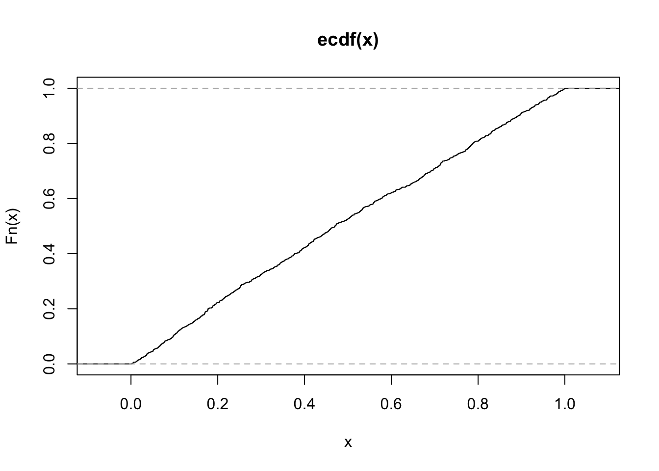
Here you can see that if \(x \sim F\), \(F(X) \sim Unif\).

x <- rnorm(1000)
plot.ecdf(x)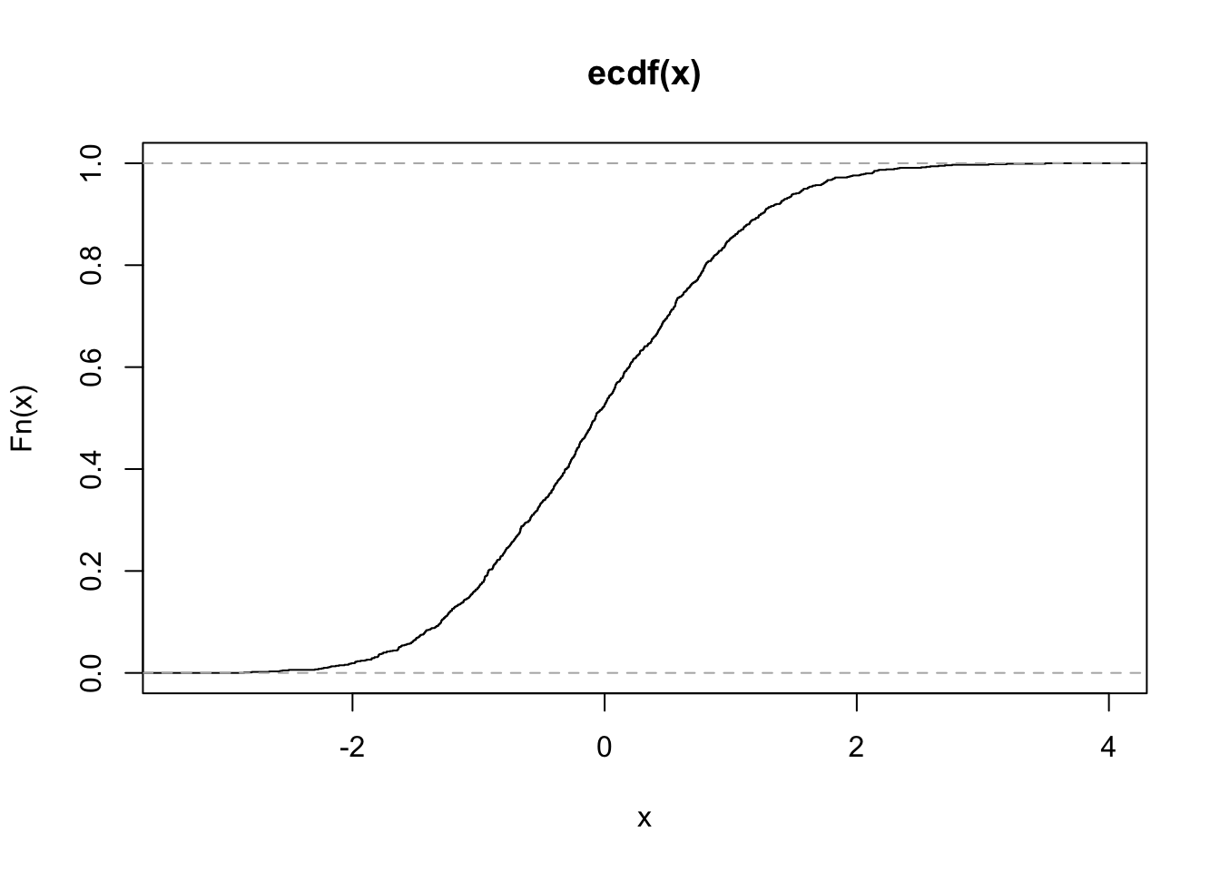

y <- pnorm(x)
plot.ecdf(y)